
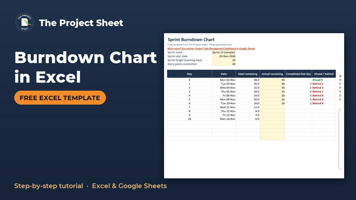
A burndown chart in Excel is a line chart that plots the story points left in a sprint against the days of the sprint, with a straight ideal line to compare against. To make one, list each sprint day, calculate the ideal remaining points, type in the actual remaining points each day, and chart the two columns as lines. The free template is below and has every formula already built.
Free download
Sprint Burndown Chart Template (Excel)
Working formulas, sample data and a How to use sheet. Opens in Excel, or import it into Google Sheets.
What the sprint burndown template does
This agile burndown template tracks one sprint on one page. You enter the sprint start date, the sprint length in working days and the story points committed. The sheet builds the ideal line, takes your daily remaining points, and shows whether you are ahead or behind.
It is made for scrum masters, team leads, project managers and freelancers who run short iterations and want a quick read on progress without opening another tool. It also suits PMP learners who want to see how an ideal vs actual burndown is calculated.
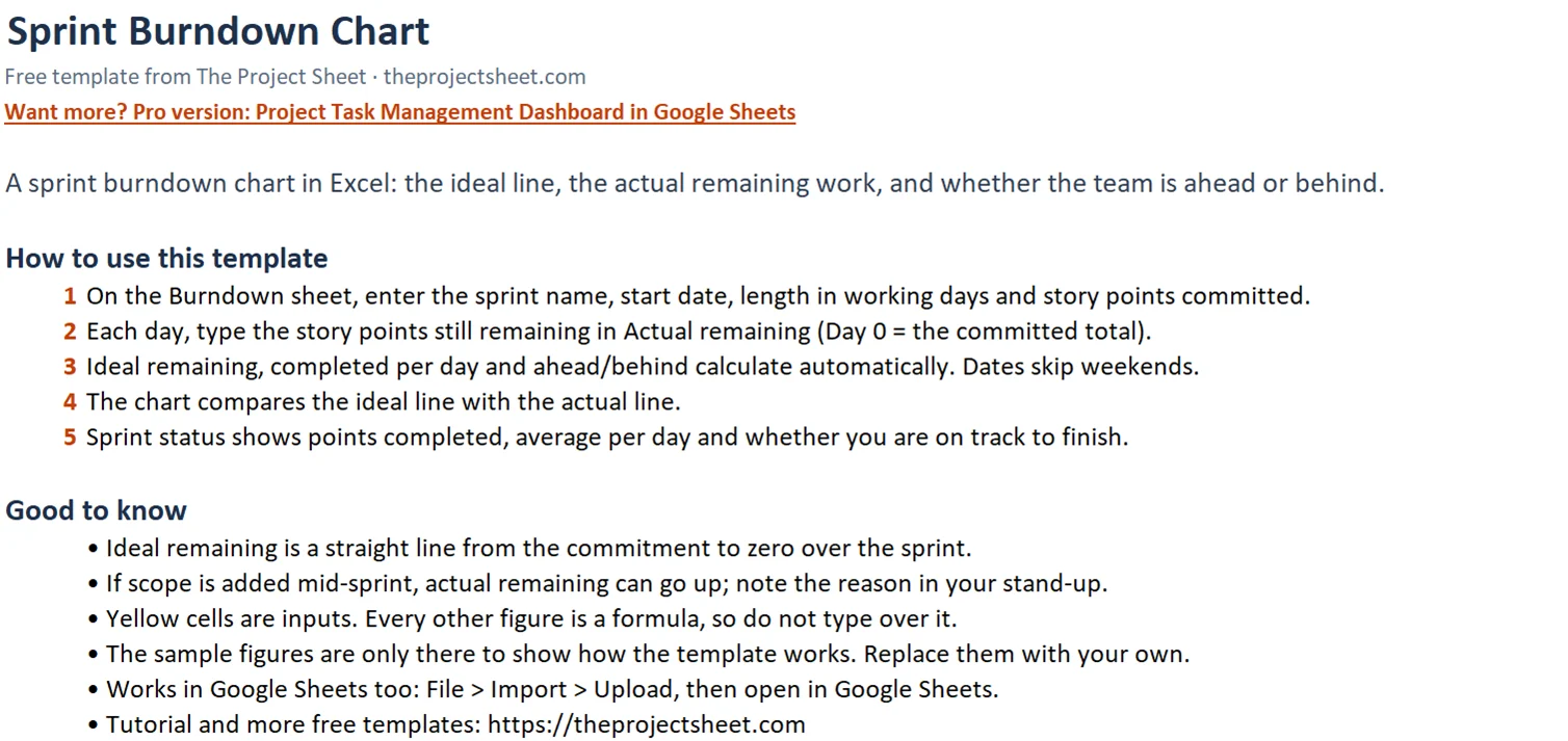
The workbook has two sheets: How to use and Burndown. All the work happens on Burndown. The How to use sheet is a short guide you can delete once you know your way around.
Why a sprint burndown chart is worth keeping
A sprint burndown chart answers one question: will the team finish what it committed to by the last day? A task list tells you what is open. The chart tells you whether the pace of work matches the plan.
Because the ideal line is straight, any gap between it and the actual line is easy to see. A gap that grows day after day is a signal to talk about scope, blockers or capacity while there is still time to act. A gap that closes tells you the team is catching up.
How to make a burndown chart in Excel, step by step
Follow these steps to build the sprint burndown chart from scratch, or use them to understand the finished template. If you only want to use the file, skip to the worked example.
Step 1: Set up the inputs in B4:B7
On the Burndown sheet, enter four values in column B:
- B4: sprint name (the sample uses "Sprint 14 (sample)")
- B5: sprint start date (02-Nov-2026, a Monday)
- B6: sprint length in working days (10)
- B7: story points committed (40)
Every other formula in the sheet reads from these four cells, so changing them updates the whole chart. Keep them in one block so anyone opening the file knows where to start.
Step 2: Build the day column (A10:A25)
Row 9 holds the headers. Rows 10 to 25 hold Day 0 up to 15 days, which leaves room for sprints of different lengths. In A10 enter 0. In the rows below, use a formula that shows the day number only while it is within the sprint length, in the form =IF(d>$B$6,"",d), where d is the day number for that row.
With a length of 10, rows past Day 10 stay blank, so the table fits the sprint automatically.
Step 3: Add working-day dates (column B)
In B10 enter:
=IF(A10=0,$B$5,WORKDAY($B$5,A10))
Day 0 returns the start date. After that, WORKDAY skips weekends. In the sample, Day 1 is Tue 03-Nov, Day 5 is Mon 09-Nov and Day 10 is Mon 16-Nov. Fill the formula down to row 25.
Step 4: Calculate the ideal line (column C)
In C10 enter:
=$B$7-$B$7/$B$6*A10
This takes the committed points and removes an equal share each day. With 40 points over 10 days the ideal runs 40, 36, 32 and so on down to 0 on Day 10. The line is straight from the commitment to zero.
Step 5: Type actual remaining points (column D)
Column D is the only column you fill in by hand. At the end of each day, type the points still not done. Day 0 is the full commitment, so enter 40. Leave future days empty so the actual line stops at today.
Do the update at the same time every day, for example right after stand-up or at the end of the working day. A steady habit keeps the line honest.
Step 6: Add points completed (column E)
In E11 subtract today’s remaining points from yesterday’s:
=D10-D11
This shows how many points the team finished that day. Fill it down alongside your data.
Step 7: Show ahead or behind (column F)
In F10 enter:
=IF(D10<=C10,"Ahead "&ROUND(C10-D10,1),"Behind "&ROUND(D10-C10,1))
Add conditional formatting so "Ahead" cells turn green and "Behind" cells turn red. Day 6 in the sample reads Behind 8.
Step 8: Build the sprint status block (I10:I15)
This block summarizes the sprint in six cells:
- Days elapsed:
=COUNT(D11:D25) - Points remaining:
=LOOKUP(2,1/(D10:D25<>""),D10:D25), which returns the last value you entered - Points completed: committed points minus points remaining
- Average points per day: points completed divided by days elapsed
- Days left:
=B6-I10 - Projected finish: compares the days needed at your current pace with the days left
The days elapsed formula starts at D11 because Day 0 is the starting point, not a day of work. That is why the sample, with values on Days 0 to 6, shows 6 days elapsed.
Step 9: Insert the line chart
Select the day, ideal remaining and actual remaining columns (A, C and D, rows 10 to 25). Choose Insert, then Line chart. Plot ideal and actual remaining by sprint day. Title the chart with the sprint name from B4 and label the axes "Sprint day" and "Story points remaining".
If Excel treats the day column as a data series instead of the horizontal axis, open Select Data and set column A as the axis labels. Then only the ideal and actual lines remain as series.
Worked example: Sprint 14 (sample)
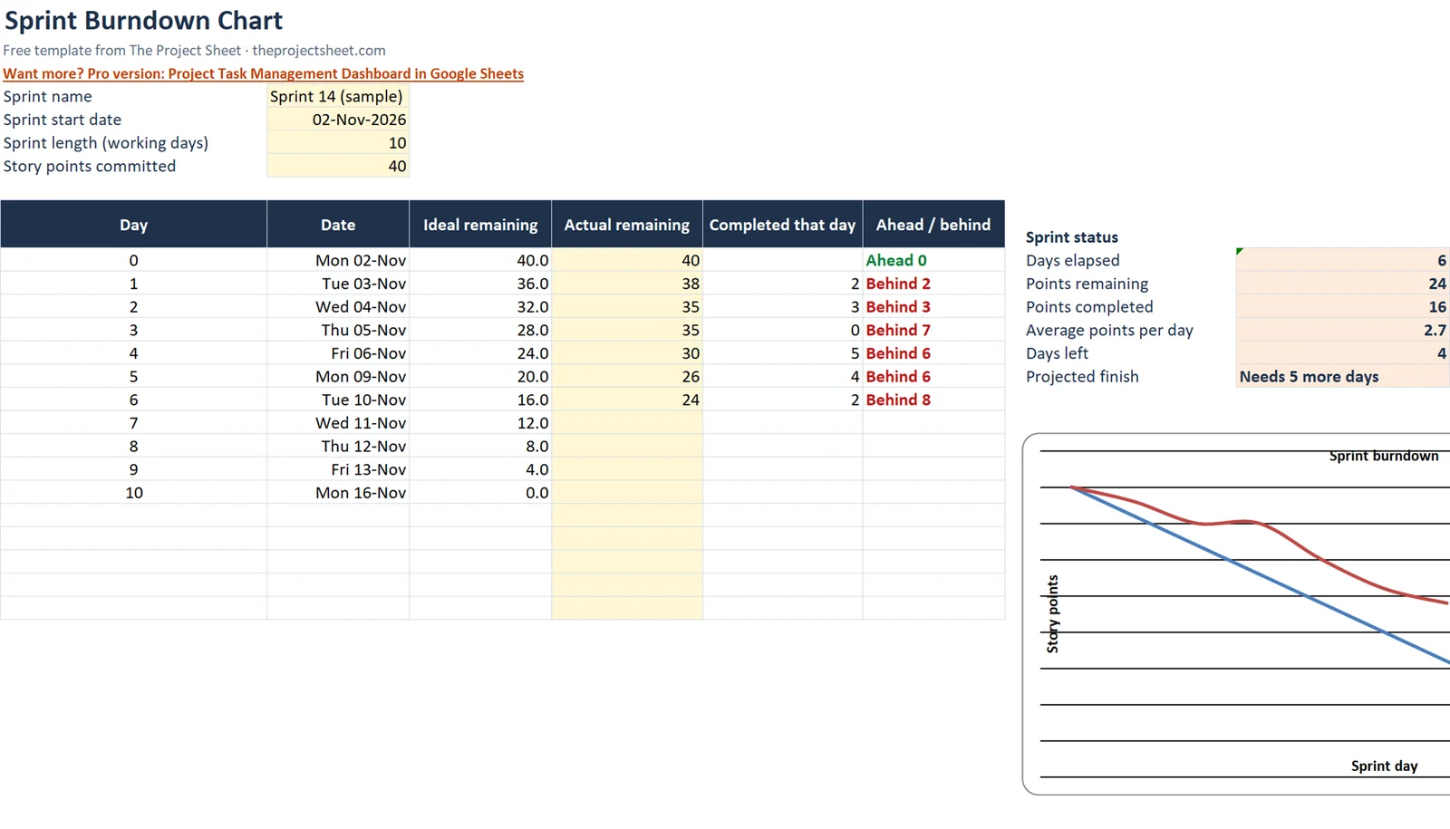
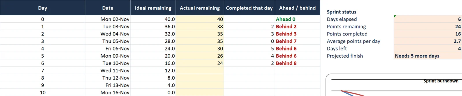
The sample sprint starts on Monday 02-Nov-2026, runs 10 working days and commits 40 story points. The team has logged Days 0 to 6.
| Day | Ideal remaining | Actual remaining | Completed that day |
|---|---|---|---|
| 0 | 40 | 40 | – |
| 1 | 36 | 38 | 2 |
| 2 | 32 | 35 | 3 |
| 3 | 28 | 35 | 0 |
| 4 | 24 | 30 | 5 |
| 5 | 20 | 26 | 4 |
| 6 | 16 | 24 | 2 |
On Day 6 the ideal line says 16 points should be left, but 24 remain. The Ahead/behind column reads Behind 8, and the actual line sits above the ideal line on the chart.
The status block gives the details: 6 days elapsed, 24 points remaining, 16 completed, and an average of 2.7 points per day. With 4 days left, the projected finish reads Needs 5 more days. At 2.67 points a day, 24 points need 9 days, and only 4 are left.
What would you do with that reading on Day 6? The numbers point to three options: cut scope, add capacity, or move the finish date. The chart does not choose for you, but it gives the team facts to discuss on day 6 rather than day 10.
How to read the chart
The ideal line is a straight diagonal from the commitment to zero. When the actual line is below it, you are ahead. When it is above it, you are behind.
A flat stretch in the actual line, like Day 3 in the sample where 0 points were completed, means no work was finished that day. Several stories may be in progress at once, with none yet done. If scope is added mid-sprint, the actual line can go up instead of down. That is a correct reading, not an error, and it is worth noting in your sprint review.
Quick reference for the chart
| What you see | What it usually means |
|---|---|
| Actual line below ideal | Ahead of plan |
| Actual line above ideal | Behind plan |
| Actual line flat | No points finished that day |
| Actual line goes up | Scope was added |
| Actual line reaches zero on or before Day 10 | Commitment met |
How to adapt the template
- Different sprint length: change B6. The table supports up to 15 days after Day 0, and the ideal line recalculates.
- New sprint: change the name, start date and points in B4:B7, then clear the actual values in column D.
- Added scope: raise that day’s remaining value in column D by the points added, and add a note beside it.
- Reporting: copy the status block into your weekly update. The Project Status Report Template: One-Page Weekly Report in Excel (Free) has room for it.
- Planning: if you need to break the work into pieces before the sprint, try the Work Breakdown Structure Template in Excel with Auto WBS Numbering (Free).
- Several teams: save one copy of the workbook per team, so each has its own inputs and its own chart.
For the bigger picture across several sprints, the Project Timeline Template in Excel: Phases and Milestones on One Page (Free) shows phases and milestones on one page.
Common mistakes
- Entering points completed instead of points remaining. Column D is what is left, not what is done.
- Filling future days with zeros. Leave them blank. Zeros make the actual line drop to the floor and break the days-elapsed count.
- Counting weekends. The date column uses WORKDAY, so the sprint length in B6 should be working days only.
- Changing a partly done story’s points. Most teams count a story only when it is done, so the line steps down rather than sliding.
- Skipping days. If you forget to log a day, the days-elapsed count and the average points per day will be off. Fill the gap before you read the status block.
- Ignoring the flat days. A run of zero-completion days is the earliest warning on the chart. Raise it at the next stand-up and record the cause in a Lessons Learned Template: Free Excel Log with Root Cause and Actions.
Excel vs Google Sheets
| Item | Excel | Google Sheets |
|---|---|---|
| WORKDAY, IF, ROUND, COUNT | Work as written | Work as written |
| LOOKUP(2,1/(…)) | Works as written | May need wrapping in ARRAYFORMULA |
| Line chart | Insert, then Line chart | Insert, then Chart, then choose Line chart |
| Green and red status | Conditional formatting | Conditional formatting |
The template is built in Excel. If you move it to Google Sheets, check the chart series and the LOOKUP cell first. Then compare the points remaining value with the last number in column D to confirm it matches.
Next step
Download the template, type your own sprint name, start date, length and committed points into B4:B7, and log your first remaining value in D10. After that, update column D once a day. If you want more templates, see the free templates page, or the start here guide if you are new to the site.
If you prefer a task-level view in Google Sheets, the Project Task Management Dashboard in Google Sheets is a paid option, and more by topic are listed under pro templates by topic.
Frequently asked questions
How do you make a burndown chart in Excel?
List the sprint days, calculate the ideal remaining points with a straight-line formula, and type the actual remaining points each day. Then select the day, ideal and actual columns and insert a line chart. The free template does all of this for you.
What is the ideal line on a sprint burndown chart?
It is a straight line from the points you committed on Day 0 down to zero on the last day. In the template the formula is =$B$7-$B$7/$B$6*A10. With 40 points over 10 days it drops 4 points a day.
What does it mean when the actual line is above the ideal line?
It means you are behind plan, because more points remain than the ideal pace allows. In the sample, Day 6 shows 24 points left against an ideal of 16, so the sheet says Behind 8.
Why can the burndown line go up?
The actual line rises when scope is added mid-sprint, because the remaining points increase. Record the added points in column D and note the reason so the team can discuss it in the sprint review.
Does the template skip weekends?
Yes. The date column uses WORKDAY, so Day 5 of the sample sprint is Monday 09-Nov and Day 10 is Monday 16-Nov. Sprint length is counted in working days.
Free download
Sprint Burndown Chart Template (Excel)
Working formulas, sample data and a How to use sheet. Opens in Excel, or import it into Google Sheets.
Want the finished version?
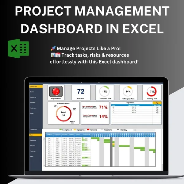
Project Management Dashboard in Excel
Progress, Gantt view, resources and risks in one Excel dashboard.
View the pro template
PK is the founder of PK: An Excel Expert and NextGenTemplates.com and a corporate trainer in Excel, VBA and Power BI. Since 2020 he and his team have built Excel and Google Sheets tutorials and templates for business users, including many project management tools.