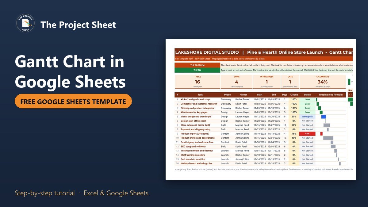
To make a Gantt chart in Google Sheets, list each task with a start date, an end date and a percent done, put one date per column across the top with SEQUENCE, then color the cells between each start and end with a conditional formatting custom formula. In the free template below the bars also change color by status, so done work is green, late work is red and work in progress is blue, with no add-ons and no chart object.
Google Sheets version
Free Gantt Chart Template for Google Sheets
Click the button to save your own copy to Google Drive. It has the 16 sample tasks, every formula, the status colors, the today line and the one-cell SPARKLINE bars.
Free download
Gantt Chart Template (.xlsx, Excel version of the Google Sheet)
Working formulas, sample data and a How to use sheet. Opens in Excel, or import it into Google Sheets.
Watch the full step-by-step video:
You can also get the free Gantt chart template, with the Google Sheets copy link, on Next Gen Templates.
What the free Gantt chart template does
The sample project is a fictional agency, Lakeshore Digital Studio, launching an online store for a home goods brand before the holiday rush. There are 16 tasks in five phases, from a kickoff workshop on 2 November 2026 to the holiday launch on 18 December 2026. Five cards at the top count the tasks, the tasks done, the tasks in progress, the late tasks and the percent complete weighted by days.
To the right sits an eight week timeline with one column per day. Every bar draws itself from the start and end dates, takes its color from the status and moves when you change a date. A red column marks today, weekends are shaded and a small arrow sits above the current day.
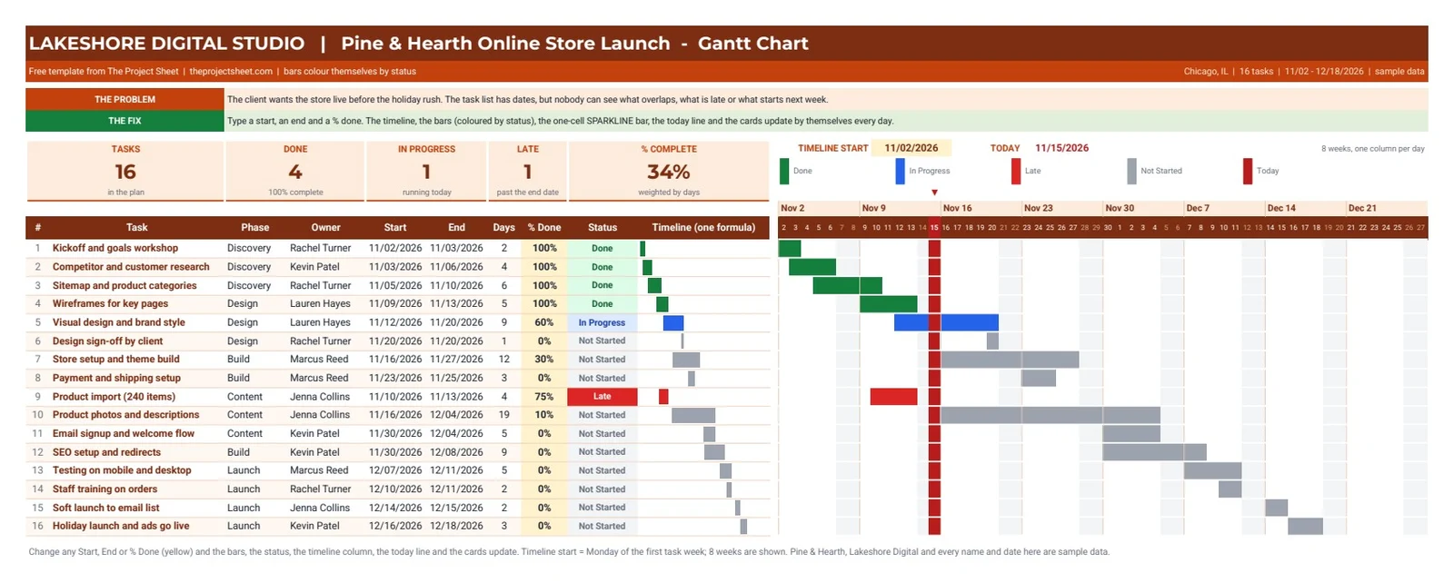
When this snapshot was taken, on 15 November 2026, the cards read 16 tasks, 4 done, 1 in progress, 1 late and 34% complete. Product import is the late one: it was due on 13 November and is only 75% done, so its bar is red. Because the status uses TODAY(), the cards and colors in your copy reflect the day you open it.
Who this template is for
- A project lead who needs a timeline the whole team can open in a browser, without a paid planning tool.
- An agency or freelancer who wants to send a client one link that shows what is done, what is late and what starts next.
- Anyone who already tracks tasks in a sheet and wants to see the overlaps, not just a list of dates.
How to make a Gantt chart in Google Sheets step by step
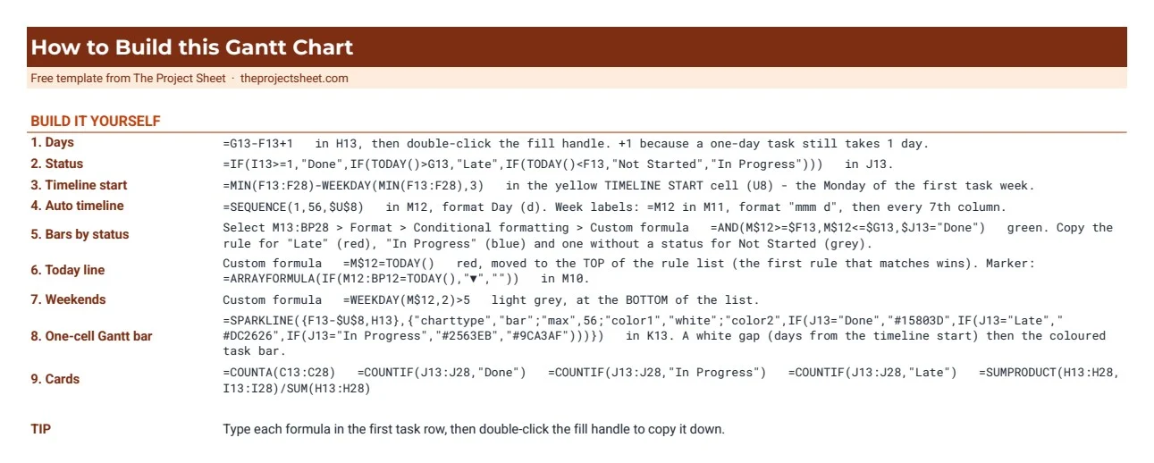
The task table starts in row 13. Column B holds the task, C the phase, D the owner, F the start date, G the end date and I the percent done. The timeline runs from column M to column BP, which is 56 days.
Step 1: Count the days of each task
In H13, subtract the start from the end and add one, because a task that starts and ends on the same day still takes a day:
=G13-F13+1
Copy it down to row 28. Store setup and theme build runs from 16 to 27 November, so it shows 12 days.
Step 2: Work out the status from the dates
The status is a formula, not a drop-down, so nobody has to remember to update it. In J13:
=IF(I13>=1,"Done",IF(TODAY()>G13,"Late",IF(TODAY()<F13,"Not Started","In Progress")))
The order of the tests matters. A task at 100% is Done whatever the dates say. Otherwise a task past its end date is Late, a task that has not reached its start date is Not Started, and anything else is In Progress. Add four Text is exactly rules on J13:J28 to color the status cells.
Step 3: Find the timeline start
The first day column should be the Monday of the week with the earliest task. In the yellow cell U8:
=MIN(F13:F28)-WEEKDAY(MIN(F13:F28),3)
WEEKDAY with type 3 counts Monday as 0, so subtracting it always lands on a Monday. The earliest task starts on 2 November 2026, which is a Monday, so the timeline starts that day.
Step 4: Build the date row with one formula
In M12, one SEQUENCE formula fills all 56 day columns:
=SEQUENCE(1,56,$U$8)
Format the row with the custom number format d so each cell shows only the day number. For the week labels, put =M12 in M11 with the format mmm d, then repeat it every seventh column. Change any start date and the whole calendar shifts with it.
Step 5: Color the bars by status
Select M13:BP28, open Format, then Conditional formatting, and choose Custom formula is. The first rule paints the done bars green:
=AND(M$12>=$F13,M$12<=$G13,$J13="Done")
The dollar signs do the work. M$12 locks the row so every cell compares its own column date. $F13 and $G13 lock the columns so every cell reads its own task row. Add the same rule for Late in red and for In Progress in blue, then one more rule without a status test in grey for Not Started:
=AND(M$12>=$F13,M$12<=$G13)
Keep the grey rule below the three colored ones. Google Sheets checks the rules from the top and stops at the first match, so a grey rule at the top would paint every bar grey.
Step 6: Add the today line and the weekend shading
Add a red rule with =M$12=TODAY() and drag it to the top of the list so it wins over the bars. Add a light grey rule with =WEEKDAY(M$12,2)>5 at the bottom so weekends are shaded only where there is no bar. For the small arrow above today, put this in M10:
=ARRAYFORMULA(IF(M12:BP12=TODAY(),"▼",""))
Step 7: Draw a Gantt bar in one cell with SPARKLINE
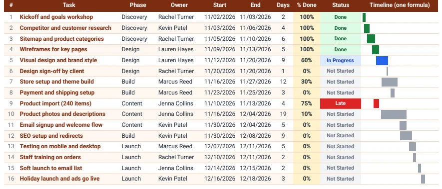
Column K shows a second, compact Gantt next to the task names. SPARKLINE with the bar chart type stacks two values: a white gap for the days before the task starts and a colored bar for its length. In K13:
=SPARKLINE({F13-$U$8,H13},{"charttype","bar";"max",56;"color1","white";"color2",IF(J13="Done","#15803D",IF(J13="Late","#DC2626",IF(J13="In Progress","#2563EB","#9CA3AF")))})
The max of 56 matches the 56 day timeline, so the small bars line up with the big ones. This column is handy when you print the task list on its own or share a narrow view on a phone.
Step 8: Add the summary cards
The cards use plain counting formulas: =COUNTA(C13:C28) for tasks, =COUNTIF(J13:J28,"Done") for done, and the same COUNTIF for In Progress and Late. Percent complete is weighted by days, so a 19 day task counts more than a one day sign-off:
=SUMPRODUCT(H13:H28,I13:I28)/SUM(H13:H28)
In the sample that gives 34%, while a simple average of the percent done column would give a different and less honest number.
Common mistakes
- Missing dollar signs. Write
M12instead ofM$12and the bars slide down diagonally, because each row compares against the wrong date row. - The grey rule on top. The first matching rule wins. Put the catch-all grey rule under the colored ones and the today rule above all of them.
- Typing the dates across the top. Typed dates do not move. Use SEQUENCE from the timeline start so the calendar follows your plan.
- Forgetting the +1 in the days. Without it a one day task shows 0 days and disappears from the weighted percent complete.
- Dates stored as text. A pasted date that sits on the left of the cell is text. Comparisons fail and the bar never shows. Retype it or use Format, then Number, then Date.
Adapt the template to your project
Make a copy, replace the tasks, owners and dates with your own and set percent done as work moves. For more than 16 tasks, insert rows inside the table and copy the formulas down. For more than eight weeks, change the 56 in SEQUENCE and in the SPARKLINE max, then stretch the conditional formatting range to the new last column. If your team works in Excel, the automatic Gantt chart in Excel uses the same idea with Excel formulas. To keep the day to day list next to the timeline, pair it with the task tracker in Google Sheets, and for a one page view of phases and milestones for a sponsor, use the project timeline template.
The Excel download above opens in Excel with the same bars, status colors and cards. SPARKLINE is a Google Sheets function, so in the Excel file the one-cell timeline in column K is drawn with REPT instead.
Want more than the free file?
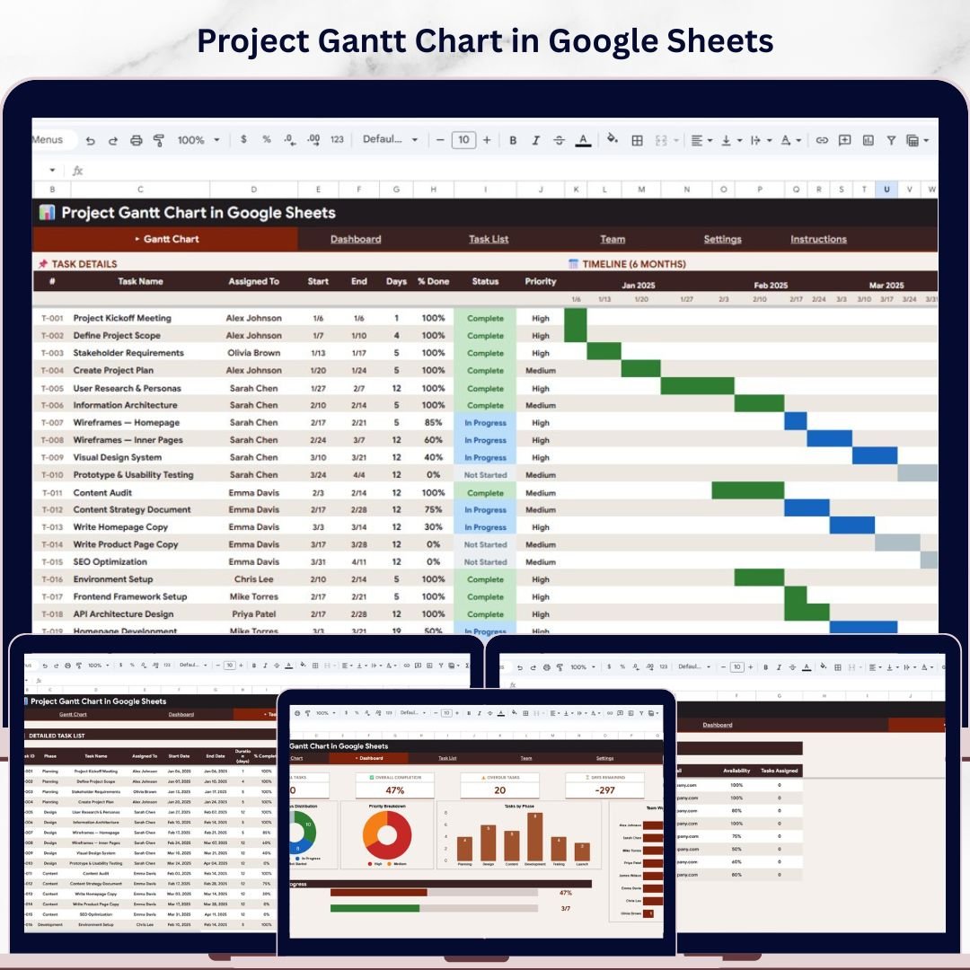
Project Gantt Chart in Google Sheets
A ready Google Sheets project Gantt with task dependencies, a KPI dashboard, team workload tracking and filters by priority, phase and team. No add-ons.
Your next step: make your copy, type your own tasks and dates, and see which bars turn red today.
Frequently asked questions
Does Google Sheets have a Gantt chart?
There is no Gantt chart type in the chart menu, but you can build one with conditional formatting. Put one date per column with SEQUENCE and color each cell that falls between a task's start and end date with a custom formula such as =AND(M$12>=$F13,M$12<=$G13).
How do I make a Gantt chart in Google Sheets?
List the tasks with start and end dates, build a date row with =SEQUENCE(1,56,start), select the grid and add conditional formatting rules with custom formulas that compare each column date with the task dates. Add a status column to color the bars by Done, Late or In Progress.
Is there a free Gantt chart template for Google Sheets?
Yes. The template on this page is free. Click Make a copy in Google Sheets to save it to your Drive, or download the Excel version. It includes 16 sample tasks, status colors, a today line and a How to Build tab.
How do I add a today line to a Google Sheets Gantt chart?
Add a conditional formatting rule on the grid with the custom formula =M$12=TODAY() and a red fill, and move it to the top of the rule list so it is checked before the bar colors.
Can I make a Gantt chart with SPARKLINE in Google Sheets?
Yes. SPARKLINE with charttype bar can stack a white gap and a colored bar in one cell, for example =SPARKLINE({F13-$U$8,H13},{"charttype","bar";"max",56;"color1","white";"color2","#2563EB"}).
Free download
Gantt Chart Template (.xlsx, Excel version of the Google Sheet)
Working formulas, sample data and a How to use sheet. Opens in Excel, or import it into Google Sheets.
Want the finished version?
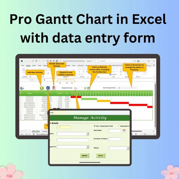
Pro Gantt Chart in Excel with Data Entry Form
Add and update activities through a form while the Gantt chart updates itself.
View the pro template
PK is the founder of PK: An Excel Expert and NextGenTemplates.com and a corporate trainer in Excel, VBA and Power BI. Since 2020 he and his team have built Excel and Google Sheets tutorials and templates for business users, including many project management tools.