How to Make a Gantt Chart in Excel (Step by Step + Free Template)

To make a Gantt chart in Excel, list your tasks with a start date and a duration, calculate each end date, then turn a grid of date columns into bars with conditional formatting. No chart object is needed: a formula rule colors each cell when its date falls between a task’s start and end. Once you know the formulas, the build takes a few minutes.

The free Gantt Chart Project Planner (Excel) is below, already set up with the formulas and rules described in this guide.

What this Gantt chart does and who it is for

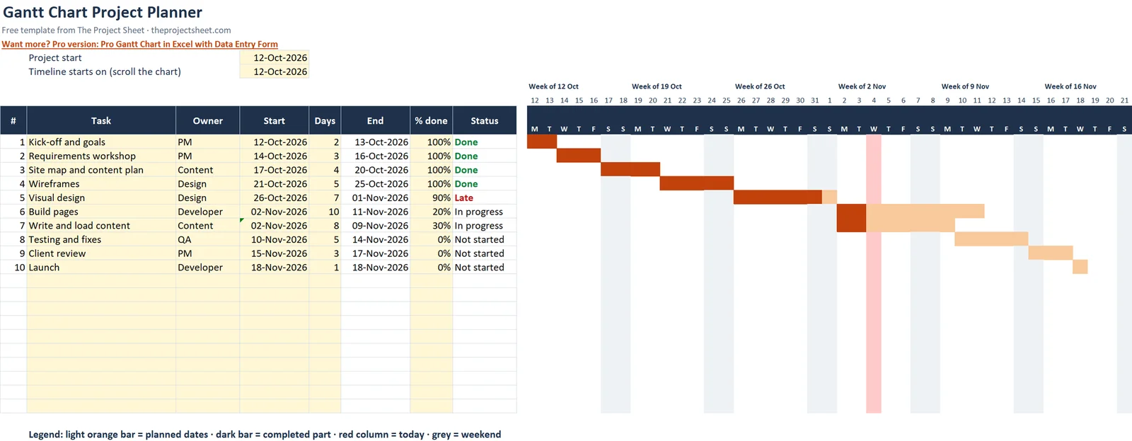
This workbook has two sheets: ‘How to use’ and ‘Gantt’. The Gantt sheet holds a task table for 20 tasks (rows 9 to 28) and a 63-day timeline to the right of it. Bars, a red today column and grey weekends are all drawn by conditional formatting.

It suits project managers, team leads, PMP learners and freelancers who need a clear schedule without installing software. If you want a gantt chart template excel users can edit without touching chart settings, this layout is easy to change, because everything is a cell and a formula.

A Gantt chart answers three questions at a glance: what is planned, when it happens, and what is running late. The sheet adds a status column so the third question is answered by a formula, not by your memory.

Why use conditional formatting instead of a chart object

Most gantt chart excel tutorials build a stacked bar chart and hide the first series. That works, but the chart sits on top of the sheet and needs its axis reset whenever dates change. Conditional formatting avoids this, because the bars are cell colors that recalculate with the data.

You also get a task table and a timeline in the same grid, so a row always lines up with its bar. Copying rows, sorting tasks and inserting a new task all behave like normal spreadsheet edits.

How to make a Gantt chart in Excel, step by step

Step 1: Set the project dates

In D4 enter the project start date. The sample uses 12-Oct-2026. In D5 enter =D4. This is the date the timeline starts on, and you can overwrite it later to scroll the chart forward.

Step 2: Build the task table

Put the headers in row 8: A is #, B is task, C is owner, D is start, E is days, F is End, G is % done and H is Status. Tasks go in rows 9 to 28. Duration in column E is in calendar days, so weekends count unless you plan around them.

Step 3: Calculate the end date

In F9 enter this formula and fill it down to row 28:

=IF(OR(D9="",E9=""),"",D9+E9-1)

The formula stays blank until a start and a duration exist. The minus 1 makes a one-day task start and end on the same day.

Step 4: Link dependencies

For a finish-to-start dependency, set the next task’s start to the day after the previous task ends. In the sample, D10 is =F9+1. Change the duration of task 1 and every task after it moves.

Tasks that run in parallel can share a start. In the sample, ‘Write and load content’ starts with ‘Build pages’ using =D14.

Step 5: Create the timeline header

The timeline has 63 day columns starting at column J. In J7 enter =$D$5. In K7 enter =J7+1 and fill right to column BT.

In row 8 show the weekday letter with =LEFT(TEXT(J7,"ddd"),1). In row 6, merge each block of 7 days and label it, for example ‘Week of 12 Oct’. Format row 7 as a short date so each column is readable.

Step 6: Add the status formula

In H9 enter this and fill down:

=IF(B9="","",IF(G9>=1,"Done",IF(AND(F9<>"",TODAY()>F9),"Late",IF(AND(D9<>"",TODAY()>=D9),"In progress","Not started"))))

The formula checks conditions in a fixed order. A task at 100% is Done, whatever the dates say. Otherwise it is Late if today is past the end date, In progress if today is on or past the start, and Not started if neither applies.

Color the Late text red and the Done text green with two simple conditional formatting rules on column H.

Step 7: Draw the bars with conditional formatting

This is the excel gantt chart conditional formatting step. Select J9:BT28, choose Home > Conditional Formatting > New Rule > Use a formula, and add four rules in this order:

1. Completed part, dark fill: =AND($D9<>"",$E9<>"",J$7>=$D9,J$7<$D9+ROUND($E9*N($G9),0))
2. Planned dates, light orange: =AND($D9<>"",$F9<>"",J$7>=$D9,J$7<=$F9)
3. Today column, red: =J$7=TODAY()
4. Weekends, grey: =WEEKDAY(J$7,2)>5

Order matters. The completed part must sit above the planned dates so the dark fill shows on top of the orange. Each rule uses the top-left cell of the range, J9, as its reference point, which is why the formulas mention J$7 and $D9.

The N($G9) part turns a blank % done cell into zero, so an empty cell never causes an error.

Step 8: Freeze the panes

Click J9 and choose View > Freeze Panes. Task names and headers then stay visible while you scroll across the timeline.

Worked example with the sample data

The sample is a 10-task website project starting on 12-Oct-2026. Each task begins the day after the previous one ends, so the bars step down the sheet like a staircase. The exception is ‘Write and load content’, which starts alongside ‘Build pages’.

Look at the Visual design task. It is 90% done, but today is past its end date. The dark fill covers the first 90% of its days (the formula rounds E*G to whole days), the orange shows the rest, and column H reads Late in red. That one row shows how the rules and the status formula work together.

Now try a change. Lengthen the first task by changing its value in column E, and watch the start of every linked task move to the right. Because D10 is =F9+1 and the later starts chain from it, you edit one number and the whole plan shifts.

Element	Where	What it does
Project start	D4	Sets the first task date
Timeline start	D5	Moves the visible window
End date	F9:F28	Start plus days minus 1
Status	H9:H28	Done, Late, In progress or Not started
Timeline dates	J7:BT7	63 consecutive days from D5
Bars	J9:BT28	Four conditional formatting rules

How to adapt it

• Change D5 to a later date to scroll the chart without moving any tasks.
• Replace the sample task names, owners and durations in rows 9 to 28. Leave unused rows empty and the formulas stay blank.
• Change the fill colors inside each rule, not the formulas.
• Add more days by copying the last timeline column to the right and extending the rule range beyond BT.
• Replace a linked start such as =F9+1 with a typed date when a task has a fixed start that does not depend on anything else.
• Update column G as work progresses. The dark fill and the status both react to it.

Pair the plan with a RACI chart template to show who is responsible for each task, and a RAID log template to track the risks and dependencies behind the dates.

If you want task status in a simpler list view, the project management template in Excel has status flags. For logging hours against these tasks, try the timesheet template in Excel.

Common mistakes

• Typing dates as text. If a start date is left-aligned, Excel may not read it as a date and the bars will not appear.
• Wrong rule order. Put the completed-part rule first, then planned dates, then today, then weekends.
• Missing dollar signs. Use $D9 and J$7 exactly as written. Without them the rule shifts as it applies across the range.
• Applying rules to one row only. The rule range must be J9:BT28.
• Hard-typing start dates. Typed dates break the dependency chain. Use =F9+1 style links where tasks depend on each other.
• Forgetting % done. Without a value in column G, no dark fill shows and the task never reaches Done.
• Entering % done as 90. Type 90% or 0.9. The formulas compare against 1, so a value of 90 would count as far more than complete.

Excel vs Google Sheets

The same formulas work in both. If you want a gantt chart google sheets version, copy the sheet over, select J9:BT28, then go to Format > Conditional formatting and choose Custom formula. Paste each of the four formulas as its own rule.

Task	Excel	Google Sheets
Add bar rules	Home > Conditional Formatting > New Rule	Format > Conditional formatting > Custom formula
Freeze panes	View > Freeze Panes at J9	Freeze rows and columns from the View menu
Formulas	Same	Same

Check the rule order in Google Sheets after pasting, since the first matching rule is the one that wins there.

Want more than a basic planner?

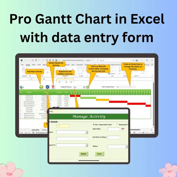
If you would rather enter tasks through a form than type into the grid, the Pro Gantt Chart in Excel with Data Entry Form is an option. You can also browse pro templates by topic.

Next step

Download the template, replace the sample tasks with your first five real ones, and set D4 to your actual start date. Once the bars look right, explore more sheets on the free templates page, or read the start here guide for a suggested order.